Land Cover Classification with eo-learn

The availability of open Earth Observation (EO) data through the Copernicus and Landsat programs represents an unprecedented resource for many EO applications, ranging from land use and land cover (LULC) monitoring, crop monitoring and yield prediction, to disaster control, emergency services and humanitarian relief. Given the large amount of high spatial resolution data at high revisit frequency, frameworks able to automatically extract complex patterns in such spatio-temporal data are required.
Last year we introduced eo-learn which aims to provide a set of tools to make prototyping complex EO workflows as easy, fast, and accessible as possible. More details are available also in our blog post Introducing eo-learn - Bridging the gap between Earth Observation and Machine Learning. After our introduction of eo-learn, the trilogy of blog posts on Land Cover Classification with eo-learn has followed. In this article, we highlight them all and invite you to read them.
Part 1: Mastering Satellite Image Data in an Open-Source Python Environment
Learn more about the initial procedures and the first steps in the machine learning (ML) pipeline for obtaining reliable results for land cover prediction. By using eo-learn, we lay down a strong and stable ground work of the full ML pipeline. It is done by preparing so-called patches of an area-of-interest, which contains all the needed information from Sentinel-2 band data. This includes cloud cover and "ground truth" reference masks. The process can run on any hardware from high-end scientific machines to personal laptops. A detailed and intuitive example in a Jupyter Notebook can help you get started with the code.
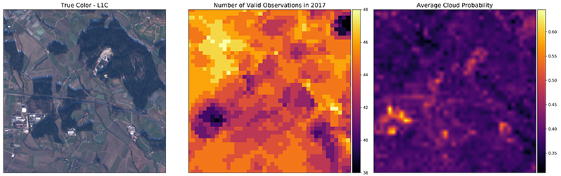
True colour image (left), map of valid pixel counts for the year 2017 (centre), and the averaged cloud probability map for the year 2017 (right) for a random patch in the AOI.
Part 2: Going from Data to Predictions in the Comfort of Your Laptop
The first blog in the series presented initial procedures for accessing and organizing the data, while in the second part we focus on training a ML classifier and using it to make prediction of land cover. We give you an example of how to use ML algorithms with open-source Python packages. You will learn that predicting land cover is not that complex by itself, but doing it properly requires validating the ML model and performing a thorough inspection of the obtained results. In the end, we use the model to predict the land cover on a country-wide scale. To compare the results of the classification with official land use data, we have made both datasets available in Geopedia, our cloud GIS web editor.
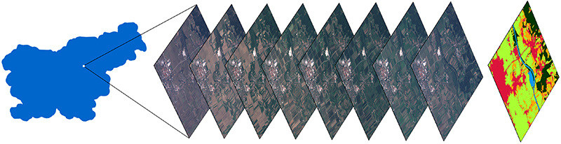
A temporal stack of Sentinel-2 images of a small area in Slovenia, followed by a land cover prediction, obtained via methods presented in this post.
Part 3: Pushing Beyond the Point of “Good Enough”
The last part of the blog series focuses on experimenting and exploring workflow variations in order to test and improve the results of the land use land cover classification for Slovenia in 2017. The experiments include testing the effects of the cloud masking and checking how different resampling techniques of the temporal interpolation affect the classification results. Additionally, we started playing around with deep learning and neural networks, taking into account both the temporal and spatial information of an area. We decided to share the whole dataset used in the blog for free, so our eo-learn users can run the experiments, improve the results and of course have fun while doing it.
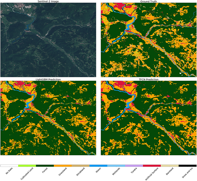
Comparison of different predictions of land cover classification. True colour image (top left), ground-truth land cover reference map (top right), prediction with the LightGBM model (bottom left), and prediction with the U-Net model (bottom right).